
Datasets in Python
- Harini Mallawaarachchi
- Jul 21, 2023
- 4 min read

Here, we'll load data from a file, filter it, and graph it. Doing so is a very important first step in order to build proper models, or to understand their limitations.
Load data with Pandas
There are large variety of libraries that help you work with data. In Python, one of the most common is Pandas. We used pandas briefly in the previous exercise. Pandas can open data saved as text files and store it in an organized table called a DataFrame.
Let's open some text data that's stored on disk. Our data is saved in a file called doggy-boot-harness.csv.
import pandas
!wget https://raw.githubusercontent.com/MicrosoftDocs/mslearn-introduction-to-machine-learning/main/graphing.py
!wget https://raw.githubusercontent.com/MicrosoftDocs/mslearn-introduction-to-machine-learning/main/Data/doggy-boot-harness.csv

# Read the text file containing data using pandas
dataset = pandas.read_csv('doggy-boot-harness.csv')

# Print the data
# Because there are a lot of data, use head() to only print the first few rows
dataset.head()
Output:
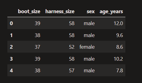
As you can see, this dataset contains information about dogs, including their doggy boot size, harness size, sex, and age in years.
Data is stored as columns and rows, similar to a table you might see in Excel.
Filter data by Columns
Data is easy to filter by columns. We can either type this directly, like dataset.my_column_name, or like so: dataset["my_column_name"].
We can use this to either extract data, or to delete data.
Lets take a look at the harness sizes, and delete the sex and age_years columns.
# Look at the harness sizes
print("Harness sizes")
print(dataset.harness_size)

# Remove the sex and age-in-years columns.
del dataset["sex"]
del dataset["age_years"]

# Print the column names
print("\nAvailable columns after deleting sex and age information:")
print(dataset.columns.values)

Filter data by Rows
We can get data from the top of the table by using the head() function, or from the bottom of the table by using the tail() function.
Both functions make a shallow copy of a section of our dataframe. Here, we're sending these copies to the print() function. The head and tail views can also be used for other purposes, such as for use in analyses or graphs.
# Print the data at the top of the table
print("TOP OF TABLE")
print(dataset.head())

# print the data at the bottom of the table
print("\nBOTTOM OF TABLE")
print(dataset.tail())
We can also filter logically. For example, we can look at data for dogs who have a harness smaller than a size 55.
This works by calculating a True or False value for each row, then keeping only those rows where the value is True.
# Print how many rows of data we have
print(f"We have {len(dataset)} rows of data")

# Determine whether each avalanche dog's harness size is < 55
# This creates a True or False value for each row where True means
# they are smaller than 55
is_small = dataset.harness_size < 55
print("\nWhether the dog's harness was smaller than size 55:")
print(is_small)

# Now apply this 'mask' to our data to keep the smaller dogs
data_from_small_dogs = dataset[is_small]
print("\nData for dogs with harness smaller than size 55:")
print(data_from_small_dogs)

# Print the number of small dogs
print(f"\nNumber of dogs with harness size less than 55: {len(data_from_small_dogs)}")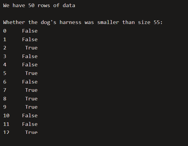
....

This looks like a lot of code, but we can compress the important parts into a single line.
Let's do something similar: restrict our data to only those with boot sizes smaller than 40.
# Make a copy of the dataset that only contains dogs with
# a boot size below size 40
# The call to copy() is optional but can help avoid unexpected
# behaviour in more complex scenarios
data_smaller_paws = dataset[dataset.boot_size < 40].copy()


# Print information about this
print(f"We now have {len(data_smaller_paws)} rows in our dataset. The last few rows are:")
data_smaller_paws.tail()
Graph Data
Graphing data is often the easiest way to understand it.
Here, we usually make our graphs using code in a custom file we've created, called graphing.py, which you can look at on our github page.
Here, we'll practice making a graph without this custom code, however.
Let's make a simple graph of harness size versus boot size for our avalanche dogs with smaller feet.
# Load and prepare plotly to create our graphs
import plotly.express
import graphing # this is a custom file you can find in our code on github

# Show a graph of harness size by boot size:
plotly.express.scatter(data_smaller_paws, x="harness_size", y="boot_size")
Create New Columns
The preceding graph shows the relationship we want to investigate for our store, but some customers might want harness-size lists in inches, not centimeters. How can we view these harness sizes in imperial units?
To do this, we will need to create a new column called harness_size_imperial and put that on the X axis instead.
Creating new columns uses very similar syntax to what we've seen before.
# Convert harness sizes from metric to imperial units
# and save the result to a new column
data_smaller_paws['harness_size_imperial'] = data_smaller_paws.harness_size / 2.54

# Show a graph of harness size in imperial units
plotly.express.scatter(data_smaller_paws, x="harness_size_imperial", y="boot_size")
We've now graphed our new column of data (harness_size_imperial) against boot size for dogs with small paws.
Summary
We've introduced working with data in Python, including:
Opening data from a file into a DataFrame (table)
Inspecting the top and bottom of the dataframe
Adding and removing columns of data
Removing rows of data based on criteria
Graphing data to understand trends
Learning to work with dataframes can feel tedious or dry, but keep going, because these basic skills are critical to unlocking exciting machine-learning techniques that we'll cover in later modules.
Comments